Tuning a data preprocessing pipeline with recipes and modelgrid

Data at a glance

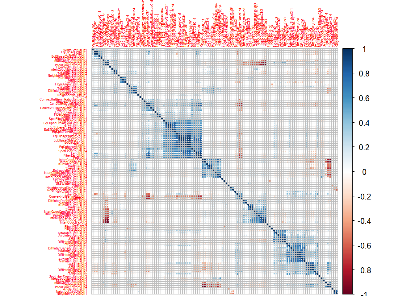
First, let us take a quick look at the data. We will do that by inspecting the between-predictor correlations of the predictors expressed by a correlation matrix of the training data set. The variables are grouped adjacent to each other according to their mutual correlations.

# Extract training data.
training <- filter(segmentationOriginal, Case == "Train")

# Extract predictors.
predictors <- training %>% select(-(c("Class", "Case", "Cell"))) 

# Identify variables with zero variance.
zero_variance_predictors <- map_lgl(predictors, ~ n_distinct(.x) == 1)

# Remove predictors with zero variance.
predictors <- predictors[, !zero_variance_predictors]

# Compute and plot a correlation matrix of remaining predictors.
library(corrplot)
predictors %>%
  cor(.) %>%
  corrplot(., order = "hclust", tl.cex = .35)

From the graph, it seems that there are groups of predictors, that have strong positive correlations (dark blue).

There can be good reasons for avoiding variables, that are highly correlated, some of them being (as stated in ‘Applied Predictive Modelling’):

• Redundant/highly correlated predictors often add more complexity than information to the model
• Mathematical disadvantages: can result in very unstable models (high variance), numerical errors and inferior predictive performance.

The aim of my modelling experiments will be to apply different preprocessing techniques in order to mitigate the potential pitfalls of the “collinearity clusters”, that we are observing amongst the field of predictors.

Create initial recipe

First, let us set up a starting point for our data preprocessing pipeline in our modeling experiments. For this purpose I apply the awesome recipes package and create a - very basic - recipe, that will serve as an anchor for my model configurations.

In this recipe I declare the roles of all variables in the data set and state, that variables with zero variances should be removed.

library(recipes)
initial_recipe <- recipe(training) %>%
  add_role(Class, new_role = "outcome") %>%
  add_role(Cell, new_role = "id variable") %>%
  add_role(Case, new_role = "splitting indicator") %>%
  add_role(-Class, -Cell, -Case, new_role = "predictor") %>%
  step_zv(all_predictors())

You can ‘prep’ the recipe and get an impression of, what it is actually doing. It seems, it removes two of the predictors due to them having variances of zero.

prep_rec <- prep(initial_recipe)
tidy(prep_rec, 1)
#> # A tibble: 2 x 1
#>   terms                       
#>   <chr>                       
#> 1 MemberAvgAvgIntenStatusCh2  
#> 2 MemberAvgTotalIntenStatusCh2

Set up a model grid

In order to organize and structure my experiments with different data preprocessing pipelines I apply my modelgrid package, that offers a framework for constructing, training and managing multiple caret models.

modelgrid separates the specification of a(ny number of) caret model(s) from the training/estimation of the model(s). By doing so, modelgrid follows the same principles as the new promising package parsnip, which is under construction.

Assume, that we want to estimate a family of Generalized Linear Models, all with different data preprocessing pipelines. I have decided on the following conditions for the model training:

• Apply a cross-validation resampling scheme with 5 folds.
• Tune the models and measure performance using the standard and highly versatile ‘Area Under the Curve’ (AUC(/ROC)) metric.

I construct a model_grid and set the settings, that by default will apply to all of my models, accordingly.

library(modelgrid)
library(caret)

models <- 
  # create empty model grid with constructor function.
  model_grid() %>%
  # set shared settings, that will apply to all models by default.
  share_settings(
    data = training,
    trControl = trainControl(method = "cv",
                             number = 5,
                             summaryFunction = twoClassSummary,
                             classProbs = TRUE),
    metric = "ROC",
    method = "glm",
    family = binomial(link = "logit")
  )

We are now ready to add individual model specifications, each with their own data preprocessing pipeline to the model grid.

Adding the first model specifications to the model grid

We will kick things off by adding the first model specification to my model grid. In this configuration I just apply our initial data preprocessing recipe and do no further. I will refer to this model as ‘baseline’.

models <- models %>%
  add_model(model_name = "baseline", 
            x = initial_recipe)

One way of dealing with the potential drawbacks of the observed “collinearity clusters” is to apply a correlation filter. The correlation filter poses a heuristic approach to dealing with highly correlated predictors. It removes the predictors with the highest between-predictor correlations one at a time, until all between-predictor correlations are below some critical threshold.

In order to do so, I extend my initial recipe with an additional step, that applies the correlation filter. Furthermore I will try out different values for the between-predictor correlation threshold value of the filter, essentially treating it as a hyperparameter.

models <- models %>%
  add_model(model_name = "corr_.7", 
            x = initial_recipe %>%
              step_corr(all_predictors(), threshold = .7)) %>%
  add_model(model_name = "corr_.8", 
            x = initial_recipe %>%
              step_corr(all_predictors(), threshold = .8)) %>%
  add_model(model_name = "corr_.9", 
            x = initial_recipe %>%
              step_corr(all_predictors(), threshold = .9))

The construction of these model specifications can - and indeed should - be parametrized. Especially if you want to try out a wider range of values for the ‘threshold’ parameter than just the three, that I have denoted here.

Great, now we have a bunch of models specifications. We will train them right away and take a first look at the results.

# Train models.
models <- models %>% train(.)
# Display resampled performance statistics of the fitted models using standard 
# functionality from the 'caret' package.
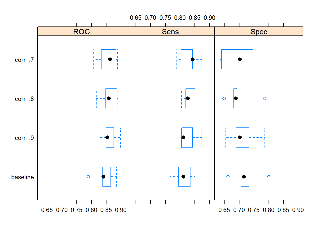
models$model_fits %>% resamples(.) %>% bwplot(.)

Judging by the resampled AUC performance statistics it seems, that there could be a case for applying a correlation filter on the set of predictors. Apparently, the model with a correlation filter with a between-predictor correlation threshold value of .7 added to the data preprocessing pipeline yields the best median resampled AUC. Of the four models, this model is by far the least complex.

We can see this by taking a look at the number of predictors, that were actually used in the final models (after removing variables with a correlation filter (if any)).

models$model_fits %>%
  map(pluck(c("recipe", "term_info", "role"))) %>%
  map_int(~ sum(.x == "predictor"))
#> baseline  corr_.7  corr_.8  corr_.9 
#>      114       60       78       93

The ‘corr_.7’ model configuration only uses 60 predictors (after removal of highly correlated predictors), hence it only estimates 61 coefficients. In contrast the ‘baseline’ model uses all predictors (except the two variables with zero variances) and estimates 115 coefficients in total making it a much more complex model (by means of a higher variance) and more prone to the risk of overfitting.

Overall it seems like applying a correlation filter with a correlation threshold value of 0.7 as part of the data preprocessing pipeline could be a good idea.

Dimensionality reduction with PCA

Another approach to dealing with highly correlated predictors is to apply a Principal Component Analysis transformation of the predictors in order to reduce the dimensions of data set. You can read more about the PCA technique here.

This approach can be tested by tweaking my initial data preprocessing recipe once again with a couple of additional steps. Before actually conducting PCA, features are centered and scaled. This is completely standard.

For the PCA transformation I vary the ‘threshold’ value, which is the fraction of the total variance of the predictors that should be covered by the components. The higher the value of ‘threshold’, the higher the number of components used.

# Extend recipe with centering and scaling steps.
rec_center_scale <- initial_recipe %>%
  step_center(all_predictors()) %>%
  step_scale(all_predictors())

# Add model specifications with pca for dimensionality reduction.
models <- models %>%
  add_model(model_name = "pca_.75", 
            x = rec_center_scale %>%
              step_pca(all_predictors(), threshold = .75)) %>%
  add_model(model_name = "pca_.85",
            x = rec_center_scale %>%
              step_pca(all_predictors(), threshold = .85)) %>%
  add_model(model_name = "pca_.95",
            x = rec_center_scale %>%
              step_pca(all_predictors(), threshold = .95))

Let us train the new model configurations and display the results.

models <- train(models)
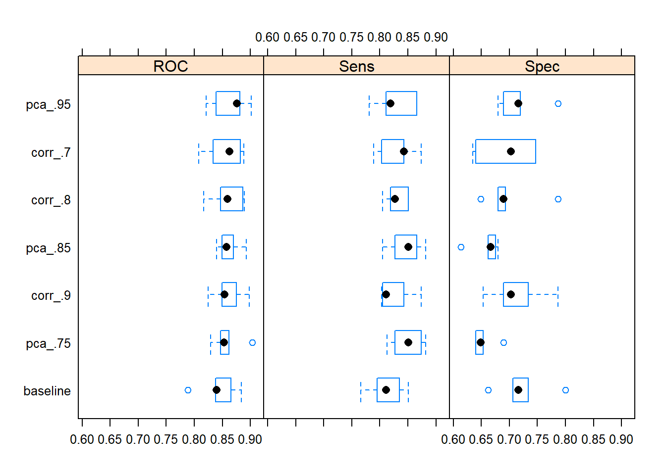
models$model_fits %>% caret::resamples(.) %>% bwplot(.)

Applying a data preprocessing pipeline with a PCA transformation capturing 95 pct. of the total variance of the set of predictors actually returns the highest resampled median value of AUC.

You can look up, how many principal components that were used in the different model configurations in order to account for the desired amount of total variance of the predictors.

models$model_fits[c("pca_.75", "pca_.85", "pca_.95")] %>%
  map(pluck(c("recipe", "term_info", "role"))) %>%
  map_int(~ sum(.x == "predictor"))
#> pca_.75 pca_.85 pca_.95 
#>      22      34      58

To summarize, adding a PCA transformation or a correlation filter to the data preprocessing pipeline seem like good ways of dealing with the “collinearity clusters” in the data set.