modelgrid is
a new package of mine, which has just made its way on to CRAN.
modelgrid offers a minimalistic but very flexible framework to create, manage
and train a portfolio of caret
models. Note, you should already be fairly familiar with the caret package
before giving modelgrid a spin.
Below I describe the key concept behind modelgrid as well as the features of
modelgrid divided into three main categories:
- Creating a model grid
- Training a model grid
- Editing and removing models from a model grid
After reading this post you should be able to grind models like never before
using the modelgrid.
Key concept behind the model grid
When facing a Machine Learning problem, you typically want to try out a lot of
models in order to find out, what works and what does not. But how can we manage
these experiments in a structured, simple and transparent way? You guessed it -
by using the modelgrid package (and yes, I am already familiar with the caretEnsemble
package, but I wanted something, that was more flexible and easier/more intuitive
to work with. Also I wanted a framework, that was pipe-friendly).
A tuning grid consists of combinations of hyperparameters for a specific model. A model grid is just an extension of that concept in the sense that it consists of - potentially many - models, each with their own tuning grid. Basically the model grid is built by providing a set of shared settings, that by default will apply to all models within the model grid, and defining the settings for the individual models in the model grid.
You can pre-allocate an empty model grid with the constructor function
model_grid and take a look at the structure.
library(modelgrid)
mg <- model_grid()

mg
#> $shared_settings
#> list()
#>
#> $models
#> list()
#>
#> $model_fits
#> list()
#>
#> attr(,"class")
#> [1] "model_grid"
An object belonging to the model_grid class has three components:
shared_settings: these are the settings, that will be shared by all models in the model grid by default. Generally, it makes sense to keep some settings fixed for all models, e.g. the choice of target variable, features, resampling scheme and sometimes also preprocessing options. By providing them as shared settings the user avoids redundant code.models: every individual model specification added to the model grid will be an element in this list. The individual model specification consists of settings that uniquely identify the indvidual model. If a setting has been set both as part of the shared settings and the settings of a given individual model specification, the setting from the individual model specification will apply for that given model.model_fits: this element contains the fitted models (one for each individual model specification), once themodel_gridhas been trained.
Creating a model grid
The first natural step of setting up the model grid is to define, which settings
should be shared by all models by default. We will use the GermanCredit data set
from the caret package as example data and do just that with the share_settings
function.
library(magrittr)
library(caret)
library(dplyr)
library(purrr)
# Load data on German credit applications.
data(GermanCredit)

# Construct empty model grid and define shared settings.
mg <-
  model_grid() %>%
  share_settings(
    y = GermanCredit[["Class"]],
    x = GermanCredit %>% select(-Class),
    preProc = "nzv",
    metric = "ROC",
    trControl = trainControl(
      method = "cv",
      number = 5,
      summaryFunction = twoClassSummary,
      classProbs = TRUE
    )
  )

purrr::map_chr(mg$shared_settings, class)
#>            y            x      preProc       metric    trControl
#>     "factor" "data.frame"  "character"  "character"       "list"
The shared_settings component of the model grid is now populated. In order to complete
the model grid we must define a set of individual model specifications, that
we would like to give a shot. A common choice of baseline model could be
a simple parametric model e.g. a Generalized Linear Model. The model specification
is added to the model grid with the add_model function.
mg <-
  mg %>%
  add_model(model_name = "Logistic Regression Baseline",
            method = "glm",
            family = binomial(link = "logit"))

mg$models
#> $`Logistic Regression Baseline`
#> $`Logistic Regression Baseline`$method
#> [1] "glm"
#>
#> $`Logistic Regression Baseline`$family
#>
#> Family: binomial
#> Link function: logit
model_grid requires a (unique) name for each individual model specification, so I
named this one ‘Logistic Regression Baseline’. If the user does not provide a name,
a generic name - ‘Model[int]’ - is generated automatically.
This is all it takes to create the smallest possible model grid with only one unique
model configuration. The model grid can be trained with the train function. For
more on this go to ‘Training a model grid’.
But a model grid with only one model specification is obviously not a really interesting use case. Let us insert another two model specifications into the model grid: a set of logistic regression models, only this time with the features being preprocessed with Principal Component Analysis.
mg <-
  mg %>%
  add_model(model_name = "Logistic Regression PCA",
            method = "glm",
            family = binomial(link = "logit"),
            preProc = c("nzv", "center", "scale", "pca")) %>%
  add_model(model_name = "Logistic Regression PCA 98e-2",
            method = "glm",
            family = binomial(link = "logit"),
            preProc = c("nzv", "center", "scale", "pca"),
            custom_control = list(preProcOptions = list(thresh = 0.98)))

mg$models
#> $`Logistic Regression Baseline`
#> $`Logistic Regression Baseline`$method
#> [1] "glm"
#>
#> $`Logistic Regression Baseline`$family
#>
#> Family: binomial
#> Link function: logit
#>
#>
#>
#> $`Logistic Regression PCA`
#> $`Logistic Regression PCA`$method
#> [1] "glm"
#>
#> $`Logistic Regression PCA`$family
#>
#> Family: binomial
#> Link function: logit
#>
#>
#> $`Logistic Regression PCA`$preProc
#> [1] "nzv"    "center" "scale"  "pca"
#>
#>
#> $`Logistic Regression PCA 98e-2`
#> $`Logistic Regression PCA 98e-2`$method
#> [1] "glm"
#>
#> $`Logistic Regression PCA 98e-2`$family
#>
#> Family: binomial
#> Link function: logit
#>
#>
#> $`Logistic Regression PCA 98e-2`$preProc
#> [1] "nzv"    "center" "scale"  "pca"
#>
#> $`Logistic Regression PCA 98e-2`$custom_control
#> $`Logistic Regression PCA 98e-2`$custom_control$preProcOptions
#> $`Logistic Regression PCA 98e-2`$custom_control$preProcOptions$thresh
#> [1] 0.98
You can of course add as many models as you like to the model grid with
the add_model function.
Training a model grid
The models from a model grid can be trained with the train function
from the caret package, for which I have implemented a S3 method for the
model_grid class.
When you call train with a model_grid, all of the individual model
specifications are consolidated with the shared settings into complete
caret model specifications, which are then trained one by one with
caret.
Consolidation of settings into complete model specifications
For a given model the model settings are consolidated with the
consolidate_model function. Let us see how this works with the three models.
For the baseline model there is no overlap between the shared settings and
the settings in the individual model specification, and hence the settings will
just be appended into one configuration.
# there are no conflicts.
dplyr::intersect(names(mg$shared_settings), names(mg$models$`Logistic Regression Baseline`))
#> character(0)

# consolidate model settings into one model.
consolidate_model(
  mg$shared_settings,
  mg$models$`Logistic Regression Baseline`
  ) %>%
  purrr::map_chr(class)
#>       method       family            y            x      preProc
#>  "character"     "family"     "factor" "data.frame"  "character"
#>       metric    trControl
#>  "character"       "list"
In case the same setting has been specified both in the shared settings of the model grid and in the individual settings for a specific model, the individual setting will apply. This is the case for the model ‘Logistic Regression PCA’, where the ‘preProc’ argument has also been defined in the model specific configuration.
# the 'preProc' setting is defined both in the shared and model specific settings.
dplyr::intersect(names(mg$shared_settings), names(mg$models$`Logistic Regression PCA`))
#> [1] "preProc"

mg$shared_settings$preProc
#> [1] "nzv"
mg$models$`Logistic Regression PCA`$preProc
#> [1] "nzv"    "center" "scale"  "pca"

# consolidate model settings into one model.
consolidate_model(
  mg$shared_settings,
  mg$models$`Logistic Regression PCA`
  ) %>%
  magrittr::extract2("preProc")
#> [1] "nzv"    "center" "scale"  "pca"
Also, if the ‘trControl’ argument is defined as part of the shared settings, the
subsettings of ‘trControl’ can be modified for a specific model with the special
setting ‘custom_control’ (which itself is given as an explicit argument to the
add_model function) in the model specific settings.
For the model ‘Logistic Regression PCA 98e-2’, the preprocessing options for PCA were adjusted with ‘custom_control’. When the model is consolidated, the model specific customizations of subsettings of the shared ‘trControl’ argument will apply.
# the 'trControl$preProcOptions$thresh' setting is defined in the shared
# settings but customized in the model specific settings.
mg$shared_settings$trControl$preProcOptions$thresh
#> [1] 0.95
mg$models$`Logistic Regression PCA 98e-2`$custom_control$preProcOptions$thresh
#> [1] 0.98

# consolidate model settings into one model.
consolidate_model(
  mg$shared_settings,
  mg$models$`Logistic Regression PCA 98e-2`
  ) %>%
  magrittr::extract2(c("trControl", "preProcOptions", "thresh"))
#> [1] 0.98
Model training
When calling the train function, the consolidate_model function is called
under the hood with all of the individual models and the shared settings, and
a set of complete caret model specifications is generated - one for each
individual model specification.
Afterwards the models are trained one by one with caret, and the fitted
models are saved in the model_fits component of the model grid.
# train models from model grid.
mg <- train(mg)

# the fitted models now appear in the 'model_fits' component.
names(mg$model_fits)
#> [1] "Logistic Regression Baseline"  "Logistic Regression PCA"
#> [3] "Logistic Regression PCA 98e-2"

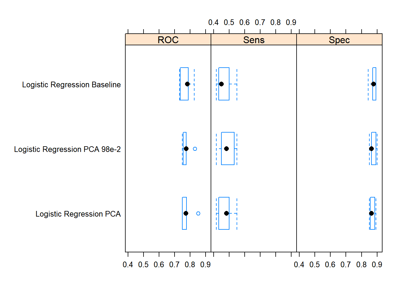
# extract performance.
mg$model_fits %>%
  caret::resamples(.) %>%
  lattice::bwplot(.)
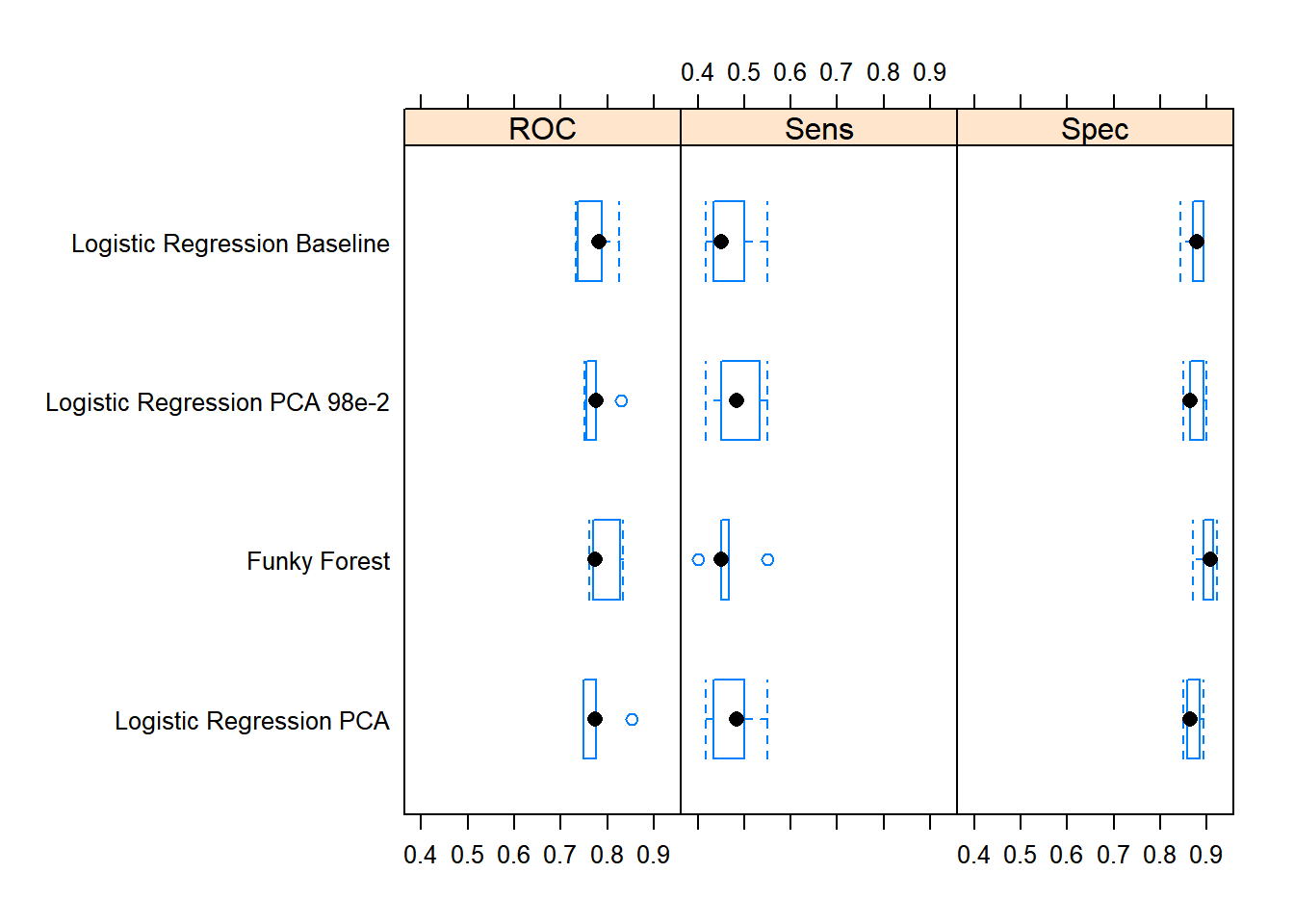
If we now add an additional models to the model grid, and call train on the model
grid again, only the new models (those that do not yet have a fit) will be trained
by default.
# train models from model grid.
mg <-
  mg %>%
  add_model(model_name = "Funky Forest",
            method = "rf") %>%
  train(.)

mg$model_fits %>%
  caret::resamples(.) %>%
  lattice::bwplot(.)
If you call train with the ‘train_all’ argument set to TRUE, all models will
be trained regardless.
Support for all train interfaces
The training of a model_grid supports both the explicit ‘x’, ‘y’ interface to train,
the ‘formula’ interface and last but not least the new powerful ‘recipe’ interface.
Let us try out the latter. First we will create a basic recipe.
# create basic recipe.
library(recipes)
rec <-
  recipe(GermanCredit, formula = Class ~ .) %>%
  step_nzv(all_predictors())
With that as a starting point I will create and train a minimal model grid as an example. I will tweak the recipe for one of the models.
mg_rec <-
  model_grid() %>%
  share_settings(
    metric = "ROC",
    data = GermanCredit,
    trControl = trainControl(
      method = "cv",
      number = 5,
      summaryFunction = twoClassSummary,
      classProbs = TRUE
    )
  ) %>%
  add_model(
    model_name = "Log Reg",
    x = rec,
    method = "glm",
    family = binomial(link = "logit")
  ) %>%
  add_model(
    model_name = "Log Reg PCA",
    x = rec %>%
      step_center(all_predictors()) %>%
      step_scale(all_predictors()) %>%
      step_pca(all_predictors()),
    method = "glm",
    family = binomial(link = "logit")
  ) %>%
  train(.)

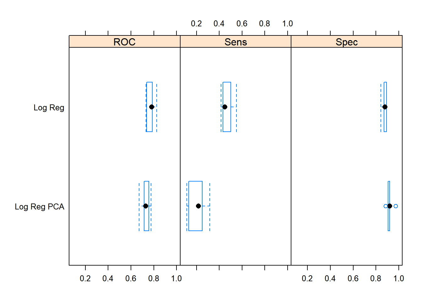
mg_rec$model_fits %>%
  caret::resamples(.) %>%
  lattice::bwplot(.)
Editing and removing models
modelgrid has a couple of functions, that makes it easy to work iteratively
with the model specifications in a model grid. If you want to modify an
existing model configuration, please use the edit_model function. Below
I use it to modify one of the generalized linear models.
# existing model configuration.
mg$models$`Logistic Regression PCA`
#> $method
#> [1] "glm"
#>
#> $family
#>
#> Family: binomial
#> Link function: logit
#>
#>
#> $preProc
#> [1] "nzv"    "center" "scale"  "pca"

# edit model configuration.
mg <-
  mg %>%
  edit_model(model_name = "Logistic Regression PCA",
             preProc = c("nzv", "center", "scale", "ICA"))
#> Model fit for Logistic Regression PCA has been deleted.

mg$models$`Logistic Regression PCA`
#> $method
#> [1] "glm"
#>
#> $family
#>
#> Family: binomial
#> Link function: logit
#>
#>
#> $preProc
#> [1] "nzv"    "center" "scale"  "ICA"
As you see, when you modify an existing model specification, any corresponding fitted model is deleted, so that everything is in sync.
You can also remove a model specification (including any fitted model) from
the model grid with the remove_model function.
names(mg$models)
#> [1] "Funky Forest"                  "Logistic Regression Baseline"
#> [3] "Logistic Regression PCA 98e-2" "Logistic Regression PCA"

# remove model configuration.
mg <-
  mg %>%
  remove_model("Funky Forest")
#> Model fit for Funky Forest has been deleted.

names(mg$models)
#> [1] "Logistic Regression Baseline"  "Logistic Regression PCA 98e-2"
#> [3] "Logistic Regression PCA"
That’s it! You should now be all set to grind models with the modelgrid.
Peace out
/smaakagen